Southern Utah County Highway GIS Analysis
Project Description
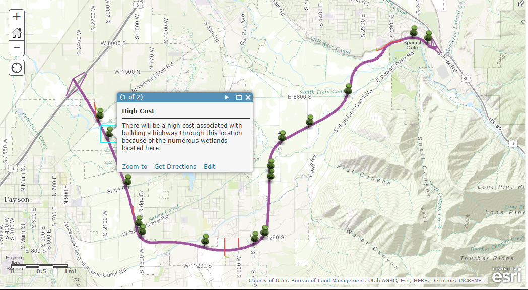
The goal of this project was to design a highway that connects a source point with five other destination points. The source point was determined by looking at where the largest growth is occurring in southern Utah County. People living in these neighborhoods will need an easier way to get to where they are going. This map shows my preferred route after taking into account all of the GIS analysis I completed. This route connects the five destinations with the source by connecting the source (south of Salem) to two major highways (I-15 north of Payson to US-6 east of Spanish Fork) that will allow the driver to travel in their intended direction. This route closely follows some of the routes created by the least cost path analysis. The only major deviation is in southwest Salem where I diverted the highway around a residential neighborhood to preserve the houses in that area.
Skills Used
- Cost Path Analysis
- Model Builder
- Raster Calculator
- ArcGIS Online
Steps Taken to Complete Project
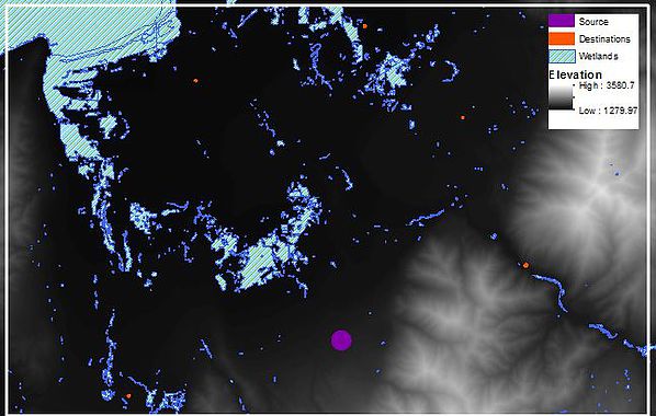
This is a map of the original wetlands and terrain data. The wetlands data was downloaded from the Utah SGID and the terrain data from the USGS National Map. The highway will need to stay away from wetlands and areas of high slope in order to keep costs low.
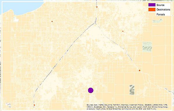
This is the original parcel data that was downloaded from the Utah County government. This data includes attributes on the price of the parcels and the land use of the parcels. Parcels that are used for commercial activities or have large building will be high cost while areas of wilderness land will be low cost. The cost of the land will also have to be taken into account since the parcels where the highway will be located will have to be purchased.
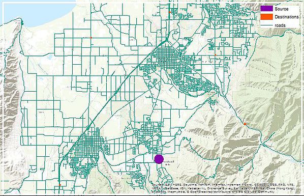
This is the road data downloaded from the Utah SGID. This data includes attributes on the types of roads and names of roads. The highway may be able to follow existing highways but it needs to stay away from local streets that would cost too much to turn into the highway.
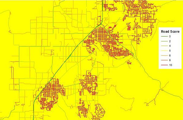
I classified the roads into different types of roads (highways, collectors, ramps, streets) and where they are located (rural, semi-rural, urban). This data was located in the attributes of the original data. I scored the roads based on these attributes. Roads with scores less than 5 are roads that would be low cost to turn into a highway. Roads with scores more than 5 would be high cost to turn into a highway. Areas with no roads were scored as a 5, meaning that it would cost more to build a highway there than to use an existing highway but it would cost less than trying to change a smaller road into a highway.
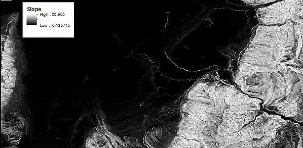
I changed the elevation data to show slope data instead. This will allow me to only choose flat slopes as places to build the highway. Steep slopes will be excluded from my model. Flatter slopes will be scored from 1 to 10, 1 being the flattest and least cost and 10 being steeper and most cost to build.
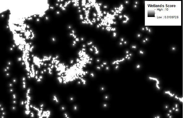
To determine a wetlands score, I used a distance decay equation to score areas close to wetlands higher than areas farther away from wetlands. This distance decay equation gives a score of 10 for the wetlands and quickly drops off to a score of 1 for locations 300 meters away from the wetlands.
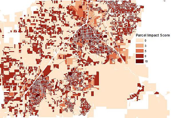
I classified parcels into different land uses and then assigned a score with each land use. Vacant lots were given the lowest scores and single family homes, apartments, churches, schools, and commercial buildings were given the highest scores. Trailer parks and parks were given scores of 5.
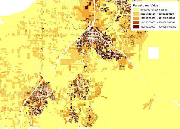
Parcels were given a land value standardized by area. To do this, I took the value of the parcel and divided it by the area of the land in acres. This gave a cost density for each parcel. This is the value that is important because if the highway is built through the middle of a large parcel, only that area will need to be purchased.
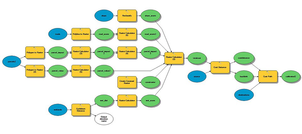
This is the model I used in ArcMap to combine the different data inputs into a total cost and then map out the least cost paths based on that total cost. Each of my inputs were converted into raster data and then I calculated a weighted average with the 6 inputs (slope score, road score, parcel impact score, parcel value score, wetlands score, and a constant score for distance). This weighted average was my total cost surface and I used GIS tools to compute the paths that cost the least amount to get from my source to each of the five destinations.
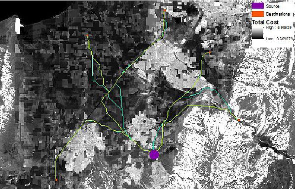
This shows the final GIS analysis, The Total Cost shows the relative cost of building a highway through each 50 square meter piece of land. Darker colors are lower cost and lighter colors are higher cost. The cost paths were created by calibrating my model and assigning different weights to the various inputs.
Back to Projects